서론
인공지능의 성능을 극대화하는 최적화 이론에 대해 심플하게 알아보자. 경사하강법부터 모멘텀, AdaGrad, RMSProp, 그리고 Adam에 이르기까지, 각 최적화 기법의 원리와 적용 방법을 설명한다. 주의해야 할 점과 취약점도 함께 다루어, 인공지능 최적화 전략에 대한 전반적인 이해를 목표로 작성하였습니다.
회귀 (regression)
회귀 분석(Regression)은 변수 간의 관계를 모델링하는 통계적 방법으로, 인공지능에서는 예측 모델을 구축하는 데 널리 사용된다. 즉, 독립 변수(X)와 종속 변수(Y) 간의 관계를 모델링하여, 새로운 독립 변수 값에 대한 종속 변수의 값을 예측하는 데 사용된다. 최적화 이론은 이 회귀 모델의 파라미터를 조정하여, 실제 값과 예측 값 사이의 차이(비용)를 최소화하는 과정에 적용된다.
예를 들어, 선형 회귀 모델에서는 경사하강법을 사용하여 비용 함수인 평균 제곱 오차(MSE)를 최소화하는 파라미터 값을 찾는다. 데이터(xi, yi) 와 예측 값(xi. axi+b)차이를 최소화 하는 (a,b)를 찾아야 한다.

경사하강법
경사하강법(Gradient Descent)은 비용 함수(Cost Function)의 기울기(Gradient)를 계산을 최소화하기 위해 파라미터를 반복적으로 조정하는 기본적인 최적화 알고리즘이다. 이 과정은 결국 비용 함수의 최소값을 찾는 것을 목표로 합니다. 즉, 함수의 극소/극대값, 경사하강법을 이용한 최솟값 찾기는 과정이다.
- 수치 미분 (h<<1 이지만 h≠0)의 경우, 실제 미분값과 수치 미분사이에 오차가 존재.
- 중심 차분을 이용한 수치 미분이 오차가 제일 적음.
- 전방/후방 차분의 경우 오차가 o(h)이지만, 중심차분의 경우 오차가 o(h)임.
경사하강법의 주의점
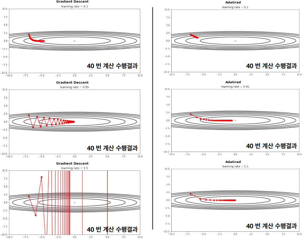
하지만 경사하강법을 사용할 때는 학습률(Learning Rate)의 선택, 지역 최소값(Local Minima)에서의 탈출, 고차원에서의 효율성 등 여러 주의점이 있다.
- 학습률이 너무 큰 경우, xn이 발산할 가능성이 큼
- 학습률이 너무 작은 경우 극솟값에 다다르는 속도가 너무 느리게 됨 (비효율적)
- 극소값에 가까워 질 수록 f’(x)<<1이 되어, 비효율적이 됨
경사하강법의 취약점
처음 시작점(보통 딥러닝에서 처음 시작점은 무작위로 주어짐) 이 최솟값보다 극소값에서 가까운 경우, 경사하강법으로 극소값에 도달하면, f′(x) = 0 이 되어, 더이상의 업데이트가 안된다.
경사하강법 개선
경사하강법의 효율을 개선하기 위한 여러 변형 기법인 모멘텀 방법, AdaGrad, RMSProp, 그리고 Adam등이 있다. 이들 각각의 알고리즘은 최적화 과정에서의 특정 문제를 해결하기 위해 고안되었습니다.
내적의 성질을 이용해 아래와 같은 분석을 할 수 있다.
- Δz가 빨리 증가하는 방향 u ∝ ∇f
- Δz가 빨리 감소하는 방향 u ∝ -∇f
경사 하강법
모멘텀 (momentum) 방법
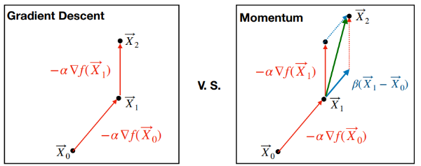
모멘텀 방법은 경사하강법에 관성의 개념을 도입한 방식이다. 경사하강법이 단순히 현재의 기울기만을 고려하여 파라미터를 업데이트하는 데 반해, 모멘텀 방법은 과거의 기울기를 어느 정도 기억하여 현재의 업데이트에 반영한다. 이를 통해 파라미터의 업데이트가 더욱 부드러워지며, 지역 최소값에 덜 민감해지고, 최적값에 빠르게 도달할 수 있다.

Adaptive Method: AdaGrad
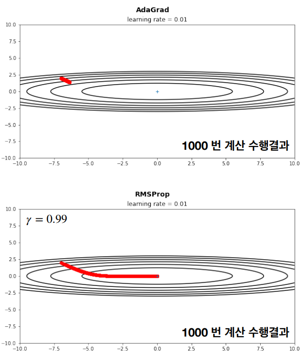
일반적인 경사하강법(Gradient Method)의 경우에는, 모든 파라메터에 대해 동일한 step-size (학습률) 이 적용하였다. 반면에 AdaGrad(Adaptive Gradient Algorithm)는 각 파라미터에 대해 개별적으로 학습률을 조정한다. 자주 업데이트되는 파라미터의 학습률은 감소시키고, 드물게 업데이트되는 파라미터의 학습률은 증가시킨다. 이로 인해 희소한 데이터에서 높은 성능을 발휘할 수 있다. 즉, AdaGrad의 핵심 개념은 과거의 모든 기울기를 제곱하여 누적시키는 것이다.
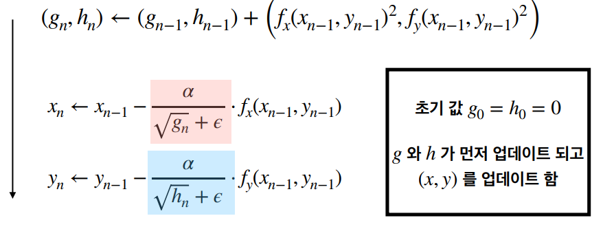
여기서 함수 f는 시간 n번째 파라미터에 대한 기울기의 제곱하였다. epsilon은 0으로 나누는 것을 방지하기 위한 작은 수이다.
Root Mean Square Propagation: RMSProp
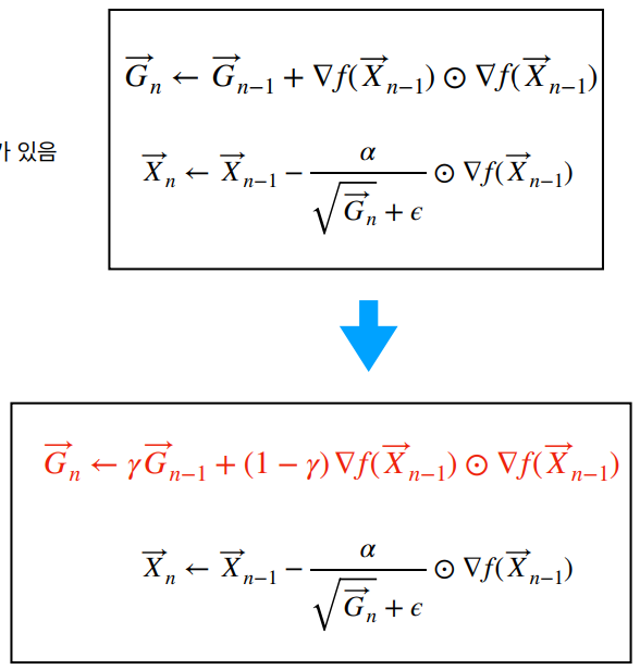
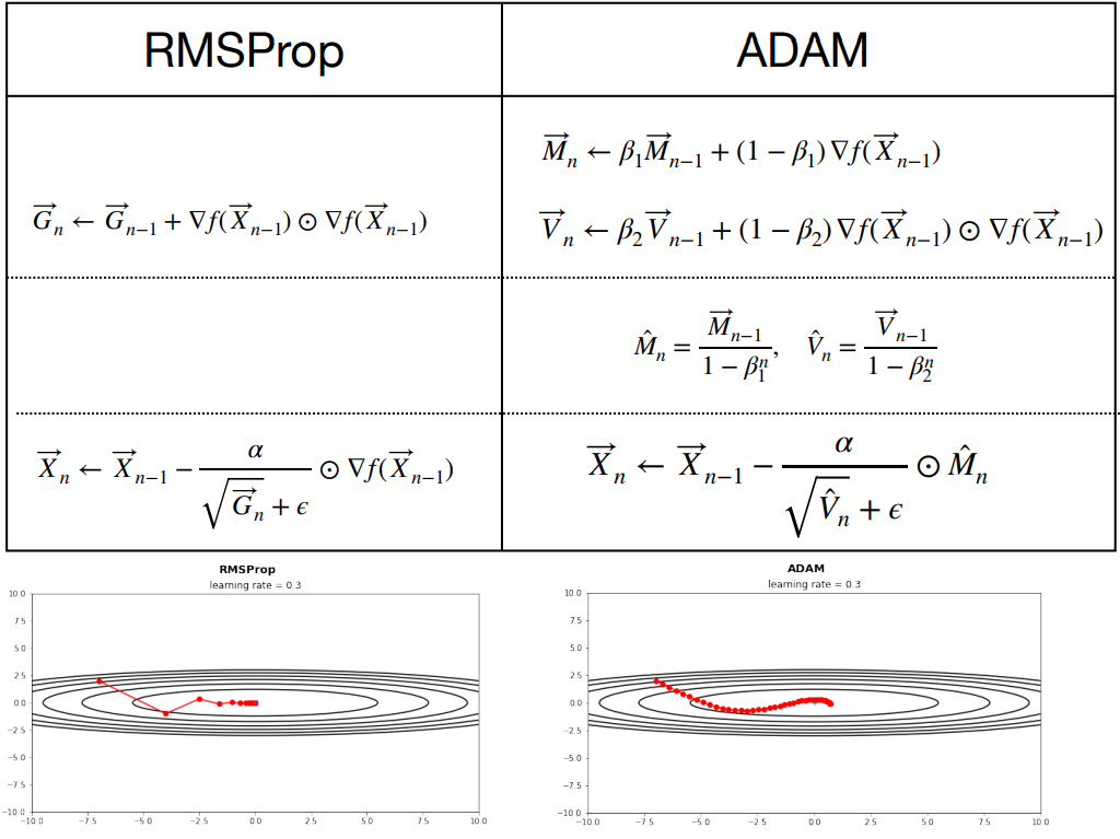
AdaGrad는 학습이 진행될 수록, 학습률이 너무 작아지는 문제가 있다. 그렇기에 AdaGrad의 문제를 해결하고자 학습이 진행될 수록, 과거의 기록의 영향을 감소시키는 RMSProp(Root Mean Square Propagation)이 탄생하였다. RMSProp은 AdaGrad의 단점을 개선한 알고리즘으로, 과거의 모든 기울기를 누적하는 대신 최근 기울기들만을 사용하여 학습률을 조정한다. 이를 통해 학습률이 너무 빠르게 줄어들어 학습이 제대로 이루어지지 않는 문제를 해결한다.
RMSProp는 다음과 같이 계산됩니다. 이 때 Gn은 γ < 1인 등비수열이다.
Adaptive Moment Estimation: Adam
Adam은 모멘텀(Momentum 혹은 AdaGrad)과 RMSProp의 개념을 결합한 알고리즘이다. Adam은 각 매개변수의 업데이트에 있어서 그 매개변수의 과거 기울기의 지수 가중 평균을 사용하며(RMSProp의 아이디어), 이를 통해 매개변수 업데이트 시 학습률의 편차를 줄인다. 또한, 과거 기울기의 지수 가중 이동 평균도 계산하여 모멘텀을 구현한다.

실제, 데이터를 가지고 함수를 최적화 시킬 때, 추출된 "표본"이 "모집단"을 잘 표현하는지가 관건이다.
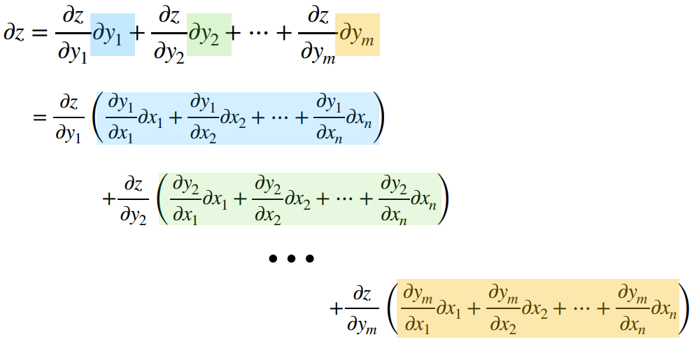
n−변수 함수의 미분
n-변수 함수란, n개의 독립 변수를 가지는 함수를 의미한다. 예를 들어, f(x_1, x_2, ..., x_n)은 n개의 독립 변수 (x_1, x_2, ..., x_n)을 가지는 함수이다. 이러한 n-변수 함수의 미분은 주로 편미분을 통해 이루어진다. 편미분은 한 변수에 대해서만 미분을 수행하고, 나머지 변수는 상수로 취급하는 미분 방법이다.
n-변수 함수 f(x_1, x_2, ..., x_n)에 대한 x_i의 편미분은 다음과 같이 표현된다.
이는 함수의 변화율이 x_i에 대해 어떻게 되는지를 나타낸다. 모든 변수에 대한 편미분을 모아놓은 것을 그래디언트(Gradient)라고 하며, 이는 다변수 함수의 방향성을 나타내는 중요한 요소이다.
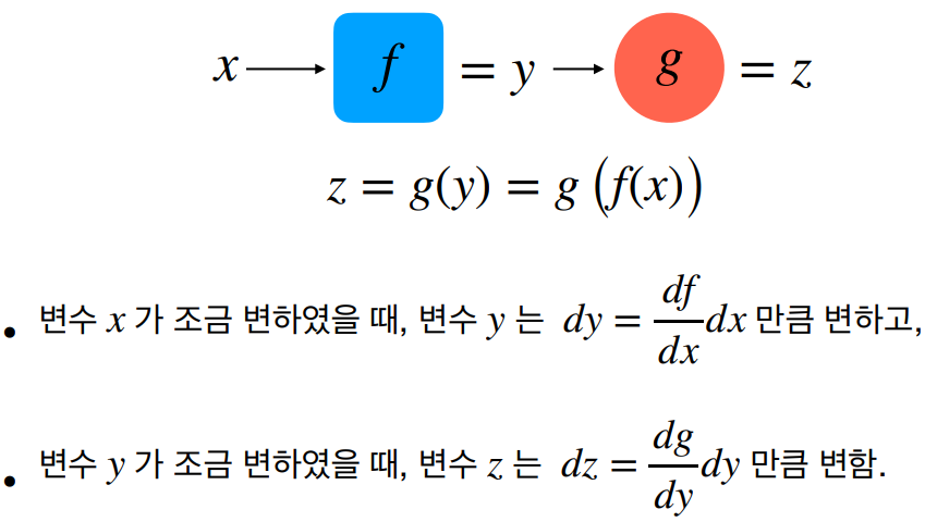
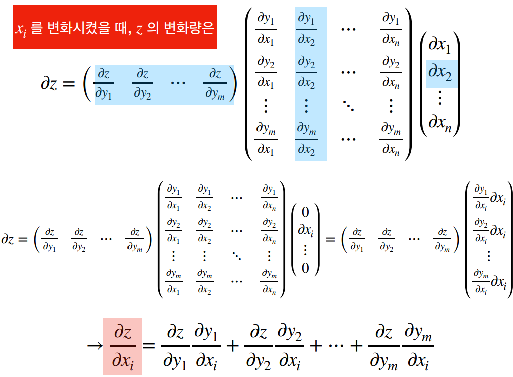
Chain Rule : 연쇄법칙
연쇄법칙(Chain Rule)은 함수의 미분을 계산하는데 중요한 역할을 하는 규칙으로, 복잡한 함수의 최적화에 필수적이다. 복잡한 함수의 미분을 계산할 때 필수적인 연쇄법칙은 심층 신경망의 역전파(Backpropagation) 알고리즘의 핵심 원리이다. 이를 통해 네트워크의 각 계층에 대한 비용 함수의 그래디언트를 효율적으로 계산하고, 이를 바탕으로 네트워크의 파라미터를 최적화할 수 있다.
주섬주섬
만약 상세히 알고 싶다면 아래 글을 참고하길 바란다.
참고
import numpy as np
from matplotlib import pyplot as plt

# 함수 f(x,y)의 Gradient (기울기 벡터) 를 grad_f(x)로 구현할 때, 이에 해당되는 수식은 다음과 같다.
def f(x,y):
     return x**2 + 1/20*y**2

# 이변수 함수의 수치 미분을 활용한 gradient (기울기 벡터) 구하는 코드
def ngrad(f,X):
    h = 1e-6
    dx = (f(X[0]+h, X[1]) -f(X[0]-h, X[1]))/(2*h)
    dy = (f(X[0], X[1]+h) -f(X[0], X[1]-h))/(2*h)
    return np.array([dx,dy])
# 경사 하강법 (Gradient decent)
class grad_decent:
def __init__(self, lr= 0.9):
self.lr = lr
def update(self, f, X):
return np.array(X) - self.lr * ngrad(f, X)
# example
lr=0.95
initial_position=(1,8) # 초기 위치를 (x,y)=(1,8) 로 설정한 경우
iter=40 # 최솟값을 찾기 위해 반복 횟수 설정
pts = [initial_position]
optimizer = grad_decent(lr)
print(pts)
pts.append(optimizer.update(f, pts[-1]))
print(pts)
print(pts[-1])
pts.append(optimizer.update(f, pts[-1]))
print(pts)
# small step_size
lr=0.95
initial_position=(1,8) # 초기 위치를 (x,y)=(1,8) 로 설정한 경우
iter=40 # 최솟값을 찾기 위해 반복 횟수 설정
pts = [initial_position]
optimizer = grad_decent(lr)
for i in range(iter):
pts.append(optimizer.update(f, pts[-1])) # append 방식을 사용하여, 계속적으로 위치 갱신
fig = plt.figure()
fig.suptitle('Gradient Descent', fontsize=14, fontweight='bold')
ax = fig.add_subplot(111)
ax.set_title('learning rate = %s' %lr)
xdata=[pt[0] for pt in pts]
ydata=[pt[1] for pt in pts]
#ax.scatter(xdata,ydata,s=10)
#ax.axis('equal')
#ax.axis([-10,10,-10,10])
plt.plot(xdata, ydata, 'o-', color="red") # 최솟값을 추적
x = np.arange(-5, 5, 0.01)
y = np.arange(-10, 10, 0.01)
X, Y = np.meshgrid(x, y)
levels = np.arange(0, 10, 2) # 등고선을 그리게 하기 위해 contour 를 설정
plt.contour(X, Y, f(X,Y),levels,colors='black') # 등고선 그림
plt.ylim(-10, 10)
plt.xlim(-5, 5)
plt.plot(0, 0, '+') # 최소값 위치
plt.show()# 모멘텀 방법
class Momentum:
def __init__(self, lr=0.01,beta=0.9):
self.lr = lr
self.beta = beta
self.v = np.zeros(2)
def update(self, f, X):
self.v = self.beta * self.v - self.lr * ngrad(f, X)
return np.array(X) + self.v
# small step_size
lr=0.09
beta= 0.95
initial_position=(1,8) # 초기 위치를 (x,y)=(1,8) 로 설정한 경우
iter=40 # 최솟값을 찾기 위해 반복 횟수 설정
pts = [initial_position]
optimizer = Momentum(lr,beta)
for i in range(iter):
pts.append(optimizer.update(f, pts[-1])) # append 방식을 사용하여, 계속적으로 위치 갱신
fig = plt.figure()
fig.suptitle('Momentum', fontsize=14, fontweight='bold')
ax = fig.add_subplot(111)
ax.set_title('learning rate=%s, beta= %s' %(lr, beta))
xdata=[pt[0] for pt in pts]
ydata=[pt[1] for pt in pts]
#ax.scatter(xdata,ydata,s=10)
#ax.axis('equal')
#ax.axis([-10,10,-10,10])
plt.plot(xdata, ydata, 'o-', color="red")
x = np.arange(-5, 5, 0.01)
y = np.arange(-10, 10, 0.01)
X, Y = np.meshgrid(x, y)
levels = np.arange(0, 10, 2) # 등고선을 그리게 하기 위해 contour 를 설정
plt.contour(X, Y, f(X,Y),levels,colors='black') # 등고선 그림
plt.ylim(-10, 10)
plt.xlim(-5, 5)
plt.plot(0, 0, '+') # 최소값 위치
plt.show()# Adaptive Method: AdaGrad
class AdaGrad:
def __init__(self, lr=0.01):
self.lr = lr
self.g = np.zeros(2)
self.epsilon= 1e-8
def update(self, f, X):
self.g = self.g + ngrad(f, X)*ngrad(f, X)
return np.array(X) - self.lr/(np.sqrt(self.g)+ self.epsilon) * ngrad(f,X)
# small step_size
lr = 0.99
initial_position=(1,8) # 초기 위치를 (x,y)=(1,8) 로 설정한 경우
iter=40 # 최솟값을 찾기 위해 반복 횟수 설정
pts = [initial_position]
optimizer = AdaGrad(lr)
for i in range(iter):
pts.append(optimizer.update(f, pts[-1])) # append 방식을 사용하여, 계속적으로 위치 갱신
fig = plt.figure()
fig.suptitle('AdaGrad', fontsize=14, fontweight='bold')
ax = fig.add_subplot(111)
ax.set_title('learning rate=%s ' %lr)
xdata=[pt[0] for pt in pts]
ydata=[pt[1] for pt in pts]
#ax.scatter(xdata,ydata,s=10)
#ax.axis('equal')
#ax.axis([-10,10,-10,10])
plt.plot(xdata, ydata, 'o-', color="red")
x = np.arange(-5, 5, 0.01)
y = np.arange(-10, 10, 0.01)
X, Y = np.meshgrid(x, y)
levels = np.arange(0, 10, 2) # 등고선을 그리게 하기 위해 contour 를 설정
plt.contour(X, Y, f(X,Y),levels,colors='black') # 등고선 그림
plt.ylim(-10, 10)
plt.xlim(-5, 5)
plt.plot(0, 0, '+') # 최소값 위치
plt.show()# RMSProp
class RMSProp:
def __init__(self, lr=0.01, gamma = 0.99):
self.lr = lr
self.gamma = gamma
self.g = np.zeros(2)
self.epsilon= 1e-8
def update(self, f, X):
self.g = self.gamma*self.g + (1-self.gamma)*ngrad(f, X)*ngrad(f, X)
return np.array(X) - self.lr/(np.sqrt(self.g)+ self.epsilon) * ngrad(f,X)
# small step_size
lr=0.9
gamma = 0.91
initial_position=(1,8) # 초기 위치를 (x,y)=(1,8) 로 설정한 경우
iter=40 # 최솟값을 찾기 위해 반복 횟수 설정
pts = [initial_position]
optimizer = RMSProp(lr, gamma)
for i in range(iter):
pts.append(optimizer.update(f, pts[-1])) # append 방식을 사용하여, 계속적으로 위치 갱신
fig = plt.figure()
fig.suptitle('RMSProp', fontsize=14, fontweight='bold')
ax = fig.add_subplot(111)
ax.set_title('learning rate=%s, gamma= %s' %(lr, gamma))
xdata=[pt[0] for pt in pts]
ydata=[pt[1] for pt in pts]
#ax.scatter(xdata,ydata,s=10)
#ax.axis('equal')
#ax.axis([-10,10,-10,10])
plt.plot(xdata, ydata, 'o-', color="red")
x = np.arange(-5, 5, 0.01)
y = np.arange(-10, 10, 0.01)
X, Y = np.meshgrid(x, y)
levels = np.arange(0, 10, 2) # 등고선을 그리게 하기 위해 contour 를 설정
plt.contour(X, Y, f(X,Y),levels,colors='black') # 등고선 그림
plt.ylim(-10, 10)
plt.xlim(-5, 5)
plt.plot(0, 0, '+') # 최소값 위치
plt.show()# Adam
class ADAM:
def __init__(self, lr=0.01, beta1 = 0.9, beta2=0.999):
self.lr = lr
self.beta1 = beta1
self.beta2 = beta2
self.m = np.zeros(2)
self.v = np.zeros(2)
self.epsilon= 1e-8
self.count=0
def update(self, f, X):
self.count+=1
self.m = self.beta1*self.m + (1-self.beta1)*ngrad(f,X)
self.v = self.beta2*self.v + (1-self.beta2)*ngrad(f,X)*ngrad(f,X)
self.mhat = self.m /(1-self.beta1**self.count)
self.vhat = self.v /(1-self.beta2**self.count)
return np.array(X) - self.lr/(np.sqrt(self.vhat)+ self.epsilon) * self.mhat
# small step_size
lr=0.2
beta1 = 0.95
beta2 = 0.995
initial_position=(1,8) # 초기 위치를 (x,y)=(1,8) 로 설정한 경우
iter=40 # 최솟값을 찾기 위해 반복 횟수 설정
pts = [initial_position]
optimizer = ADAM(lr, beta1, beta2)
for i in range(iter):
pts.append(optimizer.update(f, pts[-1])) # append 방식을 사용하여, 계속적으로 위치 갱신
fig = plt.figure()
fig.suptitle('ADAM', fontsize=14, fontweight='bold')
ax = fig.add_subplot(111)
ax.set_title('learning rate=%s, $beta_1$= %s, $beta_2$ = %s' %(lr, beta1,beta2))
xdata=[pt[0] for pt in pts]
ydata=[pt[1] for pt in pts]
#ax.scatter(xdata,ydata,s=10)
#ax.axis('equal')
#ax.axis([-10,10,-10,10])
plt.plot(xdata, ydata, 'o-', color="red")
x = np.arange(-5, 5, 0.01)
y = np.arange(-10, 10, 0.01)
X, Y = np.meshgrid(x, y)
levels = np.arange(0, 10, 2) # 등고선을 그리게 하기 위해 contour 를 설정
plt.contour(X, Y, f(X,Y),levels,colors='black') # 등고선 그림
plt.ylim(-10, 10)
plt.xlim(-5, 5)
plt.plot(0, 0, '+') # 최소값 위치
plt.show()from matplotlib import pyplot as plt
import numpy as np
# 이차원 함수 $f(x,y) 정의
fig = plt.figure(figsize=(10, 6))
x = np.arange(-10, 10, 0.01)
y = np.arange(-10, 10, 0.01)
f = lambda x, y : 1/20*x**2+ (y**2)
X, Y = np.meshgrid(x, y)
levels = np.arange(0, 10, 1.5)
plt.contour(X, Y, f(X,Y),levels,colors='black')
plt.ylim(-7, 7)
plt.xlim(-10, 10)
plt.plot(0, 0, '+')
plt.show()
# lambda 를 이용한 함수 정의
import tensorflow as tf
from tensorflow import keras
import numpy as np
weight=tf.constant([1/20, 1])
initial_position=[-7.0,2.0]
variables=tf.Variable(np.array(initial_position,dtype='float32'),trainable=True)
loss = lambda : weight*(variables**2)# Keras를 활용하여, 최솟값 찾기
lr=0.9
opt = keras.optimizers.SGD(learning_rate=lr)
iter=40
pts = [initial_position]
variables=tf.Variable([-7.0,2.0],trainable=True)
for i in range(iter):
opt.minimize(loss, var_list=variables)
pts.append(variables.numpy())
fig = plt.figure(figsize=(10, 6))
fig.suptitle('Stochastic Gradient Descent (SGD)', fontsize=14, fontweight='bold')
ax = fig.add_subplot(111)
ax.set_title('learning rate = %s' %lr)
xdata=[pt[0] for pt in pts]
ydata=[pt[1] for pt in pts]
plt.plot(xdata, ydata, 'o-', color="red")
plt.contour(X, Y, f(X,Y),levels,colors='black')
plt.ylim(-10, 10)
plt.xlim(-10, 10)
plt.plot(0, 0, '+')
plt.show()# SGD 에 Momentum 방식을 더한 최솟값 찾기
lr=0.1
opt = keras.optimizers.SGD(learning_rate=lr ,momentum= 0.9)
iter=40
pts = [initial_position]
variables=tf.Variable([-7.0,2.0],trainable=True)
for i in range(iter):
opt.minimize(loss, var_list=variables)
pts.append(variables.numpy())
fig = plt.figure(figsize=(10, 6))
fig.suptitle('SGD with Momentum', fontsize=14, fontweight='bold')
ax = fig.add_subplot(111)
ax.set_title('learning rate = %s with momentum = %s' %(lr, 0.9))
xdata=[pt[0] for pt in pts]
ydata=[pt[1] for pt in pts]
plt.plot(xdata, ydata, 'o-', color="red")
plt.contour(X, Y, f(X,Y),levels,colors='black')
plt.ylim(-10, 10)
plt.xlim(-10, 10)
plt.plot(0, 0, '+')
plt.show()# Adagrad 방식을 활용한 최솟값 찾기
lr=0.95
opt = keras.optimizers.Adagrad(learning_rate=lr, initial_accumulator_value=0)
iter=40
pts = [initial_position]
variables=tf.Variable(np.array(initial_position,dtype='float32'),trainable=True)
for i in range(iter):
opt.minimize(loss, var_list=variables)
pts.append(variables.numpy())
fig = plt.figure(figsize=(10, 6))
fig.suptitle('Adagrad', fontsize=14, fontweight='bold')
ax = fig.add_subplot(111)
ax.set_title('learning rate = %s' %lr)
xdata=[pt[0] for pt in pts]
ydata=[pt[1] for pt in pts]
plt.plot(xdata, ydata, 'o-', color="red")
plt.contour(X, Y, f(X,Y),levels,colors='black')
plt.ylim(-10, 10)
plt.xlim(-10, 10)
plt.plot(0, 0, '+')
plt.show()# RMSprop을 사용한 최솟값 찾기
lr=0.3
opt = keras.optimizers.RMSprop(learning_rate=lr,rho=0.99)
iter=40
pts = [initial_position]
variables=tf.Variable(np.array(initial_position,dtype='float32'),trainable=True)
for i in range(iter):
opt.minimize(loss, var_list=variables)
pts.append(variables.numpy())
fig = plt.figure(figsize=(10, 6))
fig.suptitle('RMSProp', fontsize=14, fontweight='bold')
ax = fig.add_subplot(111)
ax.set_title('learning rate = %s' %lr)
xdata=[pt[0] for pt in pts]
ydata=[pt[1] for pt in pts]
plt.plot(xdata, ydata, 'o-', color="red")
plt.contour(X, Y, f(X,Y),levels,colors='black')
plt.ylim(-10, 10)
plt.xlim(-10, 10)
plt.plot(0, 0, '+')
plt.show()# ADAM을 사용한 최솟값 찾기
lr=0.3
opt = keras.optimizers.Adam(learning_rate=lr,beta_1=0.9, beta_2=0.999)
iter=40
pts = [initial_position]
variables=tf.Variable(np.array(initial_position,dtype='float32'),trainable=True)
for i in range(iter):
opt.minimize(loss, var_list=variables)
pts.append(variables.numpy())
fig = plt.figure(figsize=(10, 6))
fig.suptitle('ADAM', fontsize=14, fontweight='bold')
ax = fig.add_subplot(111)
ax.set_title('learning rate = %s' %lr)
xdata=[pt[0] for pt in pts]
ydata=[pt[1] for pt in pts]
plt.plot(xdata, ydata, 'o-', color="red")
plt.contour(X, Y, f(X,Y),levels,colors='black')
plt.ylim(-10, 10)
plt.xlim(-10, 10)
plt.plot(0, 0, '+')
plt.show()기계 학습 4. 회귀(Regression) 분석
서론 학습 모델 중에서 가장 심플한 선형 회귀(Linear Regression) 모델에 대해 우선 살펴보자. 해당 모델은 크게 두 분류로 구분할 수 있다. 훈련 세트에 대해 모델을 가장 잘 맞게 하는 모델 파라미
jinger.tistory.com
Keras documentation: Optimizers
Optimizers Usage with compile() & fit() An optimizer is one of the two arguments required for compiling a Keras model: import keras from keras import layers model = keras.Sequential() model.add(layers.Dense(64, kernel_initializer='uniform', input_shape=(10
keras.io
'컴퓨터공학 > AI' 카테고리의 다른 글
| 인공지능 4. 다층 신경망 (0) | 2024.04.11 |
|---|---|
| 인공지능 3. 단층 신경망 (1) | 2024.04.07 |
| 인공지능 1. 퍼셉트론 (0) | 2024.04.01 |
| AI를 배우기 전 행렬 이론 기초 (2) | 2024.03.14 |
| 기계학습 12. Convolutional Neural Networks(CNN) (0) | 2023.12.12 |


댓글